All guides › Statistics and interpreting results
What can a histogram tell me about my laboratory data?
A histogram shows how often results fall into successive ranges. It can reveal where most observations sit, how far they spread and whether there are gaps, long tails or clusters worth investigating.
Worked example at a glance
48 results
Receipt-to-authorisation times
5 minutes
Width of each interval
2 workflows
24 results from each
Read the axes before interpreting the shape
Each bar counts observations in a range of values, called a bin. In this guide, every bin is five minutes wide, so taller bars contain more results. Adjacent bins represent adjacent ranges on a numerical scale. [1]
Start by looking at where the results are concentrated, then look for gaps, tails and clusters. Bin width and bin boundaries affect how the same data look. Very wide bins can hide features, while very narrow bins can make a modest sample look fragmented. If a feature matters, see whether it remains visible with another sensible choice of bins. [1]
See what changes when you label the workflows
A fictional laboratory records 48 receipt-to-authorisation times for one test. In the pooled histogram, results gather in two separate bands.

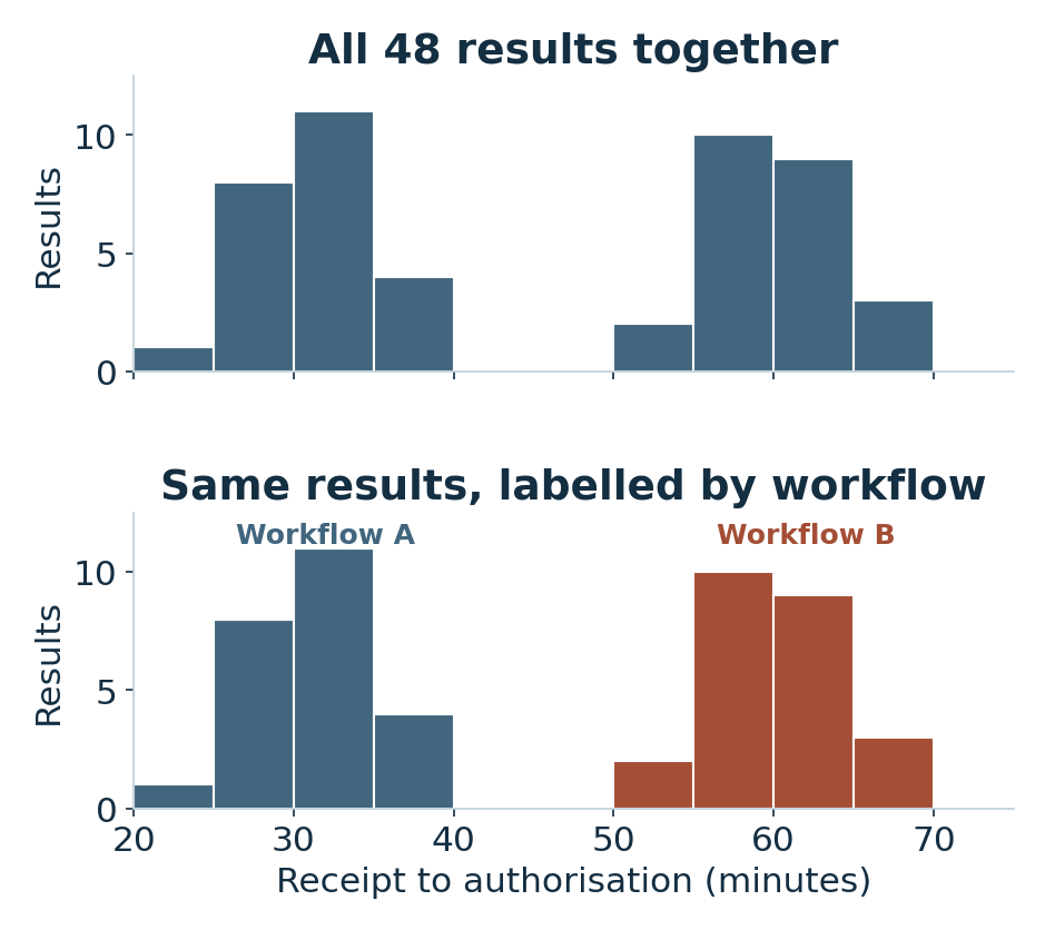
The gap prompts a question about whether the times came from different processes. When the laboratory labels each observation by workflow, the shorter times belong to workflow A and the longer times to workflow B in this set.
The split gives a plausible explanation for the two clusters. To understand the difference, the laboratory would still need information about how the cases were routed, how the timestamps were captured and what else varied between workflows.
Use the shape to choose the next view
The overall range in the table summarises the shortest and longest observed times. The histogram shows that the times did not fill that range evenly.
| Observations | Count | Observed range |
|---|---|---|
| All results | 48 | 24–68 min |
| Workflow A | 24 | 24–39 min |
| Workflow B | 24 | 53–68 min |
A histogram rearranges the observations by value. It loses their time order. To see whether turnaround changed after an event or varied by day, plot the original times in chronological order.
When comparing separate histograms, use matching bin boundaries and axis scales. If groups are very different in size, proportions can make their shapes easier to compare. Show the sample sizes as well.
Describe what the graph showed
State which observations were included and which bin width you used. Separate the feature in the histogram from the explanation you plan to check.
Example wordingThe 48 recorded times formed two clusters using five-minute bins. In these observations, the shorter cluster belonged to workflow A and the longer cluster to workflow B.
Member Learning
Plan a laboratory study and prepare your data
Work through a laboratory study, from planning and checking the source data to summarising results and explaining their limits.
Sources and related reading
- NIST/SEMATECH e-Handbook · Histogram · Explains how to read the centre, spread, tails and modes in a histogram.
Read when to use SD, CV, standard error or a confidence interval
By Stephen MacDonald · Suggest a correction · Back to Find a guide